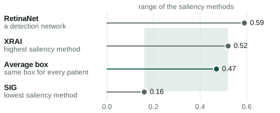
A clinician shown a heatmap of what a medical imaging model looked at cannot tell from the picture whether the heatmap is true. Such a heatmap is called a saliency map. Arun and colleagues (2021) compared saliency maps on chest X-rays with boxes that radiologists drew around pneumonia. As a baseline, they averaged all the boxes into one average box and used it as the explanation for every patient.
That baseline holds no information about the individual patient, and it beat almost every saliency method. It scored 0.47 on AUPRC, the area under the precision-recall curve, here a measure of overlap with the radiologists’ boxes. Every saliency method tested scored lower except XRAI, at 0.52.
XRAI then failed a test that randomises the numbers a model has learned, on both pneumonia and pneumothorax, a collapsed lung. On pneumonia, two other methods scored higher on randomised models than on trained ones. Overlap with an expert therefore did not track what the model had learned.
No single test proves that a model is interpretable. A defensible claim names the explanation, the model, the purpose and the tests the explanation passed.
A claim of interpretability is a claim about a mechanism: the model’s output depends on the thing the explanation names. Lipton (2018) showed that “interpretable” covers several motivations that conflict, and Doshi-Velez and Kim (2017) argued that evaluation needs a named task.
Overlap with experts
Overlap with an expert is a weak test, because the average box scores well on it and a good model can score badly. Saporta and colleagues (2022) reported a model that detected support devices, such as tubes and lines, on chest X-rays at AUROC 0.969. AUROC is the chance that a model ranks a positive case above a negative one. Grad-CAM, a saliency method, overlapped the true location at a mean intersection over union of 0.163, where 1 is perfect overlap.
The authors said it is “difficult, if not impossible” to know whether such poor overlap comes from the model or from the saliency method.
Dependence on the model
An explanation that stays the same when the model is destroyed cannot be explaining that model. Adebayo and colleagues (2018) built a randomisation test on this idea. It replaces the numbers a model has learned, its weights, with random ones, layer by layer, and it also retrains the model on shuffled labels, the answers it learns from.
The saliency methods Gradients and Grad-CAM passed, while Guided Backpropagation and Guided Grad-CAM failed. An edge detector, which uses no model at all, also produced maps that look like saliency maps.
The randomisation test gives a pass or a fail and cannot rank methods. Binder and colleagues (2023) proved that random noise scores well if similarity to the original map is used as a ranking, and they kept the test as a binary one. A pass shows only that the explanation depends on the model in some way.
Removing what the explanation points at
If an explanation names the important pixels, removing them should lower accuracy. Hooker and colleagues (2019) tested this with ROAR, which removes pixels and then retrains the model, so that the drop cannot come from a model confused by altered images. On ImageNet, a large photograph benchmark, retraining with 90 percent of pixels replaced at random gave 63.53 percent accuracy, down from 76.68 percent on the original data.
Gradients, Integrated Gradients, Guided Backpropagation and classic SmoothGrad did not beat that random replacement, while SmoothGrad-Squared and VarGrad far outperformed it. The pixels that those four methods ranked highest appeared to be no more informative than random pixels. The authors noted that ROAR can miss redundant information, which stays available to the retrained model after one copy is removed.
The pattern of removed pixels, called a mask, can itself carry information. Rong and colleagues (2022) trained a classifier, a model that sorts images into classes, on the masks alone, with no pixels. For the saliency method IG-SG on CIFAR-10, a benchmark of small photographs, it reached almost 80 percent accuracy, compared with 85 percent on full images, because the shape of a mask can reveal the class. Their removal test, ROAD, avoids this by filling removed pixels from their neighbours.
Blurring a map also changes the score. A workshop paper by Song and colleagues blurred saliency maps with max-pooling or a Gaussian filter. Accuracy after removal fell further, which counts as a better score, in at least 74 of 81 comparisons on ROAR and ROAD. The authors called this “a persistent blurriness bias”. A blurred map may also be a more accurate map, and these scores alone cannot separate the two.
Planted signals
A planted signal fixes the right answer in advance. Zhou and colleagues (2022) reassigned the labels of bird images so that only a signal they added to the images could predict the labels, and 70 percent of runs passed 95 percent accuracy on test images, which showed that those models had learned the signal. A correct method should then put almost all of its map on the planted signal.
None of the five saliency methods did this consistently. SHAP, which estimates each input’s contribution to the output, did best, at an average of 69 percent.
Planted signals can also measure false alarms, as Adebayo and colleagues (2022) showed by including clean models that do not rely on the signal. From those models and usefulness ratings by 200 participants, they concluded that even with prior knowledge, “only the concept activation approach, for visible spurious signals, is effective”. That approach tests whether a named human concept affects the output.
Shortcuts in real data
An explanation can find a real flaw when someone then changes the input and measures the output. COVID-19 models on chest radiographs in DeGrave and colleagues (2021) reached AUROC 0.992 on images from their training sources, which fell to 0.76 on images from other sources. Saliency maps pointed at text markers and image borders, and edited images confirmed the shortcut.
Concepts
Concept bottleneck models, from Koh and colleagues (2020), compute their prediction from named human concepts, so that a clinician can correct a concept and watch the output change. In a simulation on grading knee osteoarthritis, supplying the true values of 2 concepts cut the root mean square error, the typical size of an error, from above 0.4 to about 0.3.
A concept’s name can misstate what it carries. Mahinpei and colleagues (2021) used handwritten digits with no fours or fives, and concepts “is a four” and “is a five”. A classifier for odd or even digits, given the predicted probabilities of those concepts, reached 69 percent accuracy where 50 percent was expected, so the probabilities carried information the names did not describe.
An adversary
The tests so far assume that nobody is trying to mislead. LIME explains a prediction by fitting a small model to altered copies of an input. Slack and colleagues (2020) built a biased model with a scaffold that detects those copies and answers them with an unbiased model.
On COMPAS, a criminal justice dataset, the scaffold kept one sensitive input out of LIME’s top rank on all test points. SHAP was harder to fool. The sensitive input stayed out of its top rank on 84 percent of test points when one input was targeted and 67 percent when two were. The scaffold also matched the biased model on 91 percent of predictions, against 100 percent for LIME. A vendor who supplies both the model and the evidence could build such a scaffold.
People
A study of explanations in use needs a study arm where the model is wrong, because the question is whether people overrule it. Senoner and colleagues (2024) reported that saliency maps raised radiologists’ balanced accuracy, the mean accuracy across classes, by 4.7 percentage points. Disease detection did not change (90.4 percent in both arms). The gain came from following correct model predictions more (82.1 against 72.4 percent).
Radiologists with saliency maps also overruled fewer wrong predictions (50.8 against 57.7 percent).
Wrong advice can lower clinicians’ accuracy with or without an explanation. In Jacobs and colleagues (2021), on simulated antidepressant advice, explanations listing the inputs behind wrong advice reduced accuracy against decisions made with no advice. In Gaube and colleagues (2021), no explanation was shown, and diagnostic accuracy fell when chest X-ray advice was wrong, whatever its stated source.
Alternatives to explanation
Two published positions avoid post hoc explanation, meaning explanation added after training. Ghassemi and colleagues (2021) held that explanations can be useful for development and audit but are “rarely informative with respect to individual decisions”. In the absence of suitable methods, they advocated validation, which tests the model’s performance directly.
Rudin (2019) argued for models that are interpretable by construction. Such a model still has to show that its output depends on its structure.
A test on my own model
My ECG model, under review, predicts atrial fibrillation, an irregular heart rhythm, from an ECG, a recording of the heart’s electrical activity. It computes its risk score through factors, learned patterns defined over frequency and over ECG lead, one of the electrode views of the heart. I ranked frequency bins, narrow frequency bands, and leads by how much AUROC fell when each was zeroed, on data held out from training.
On that data, zeroing the 10 top-ranked inputs lowered AUROC by 0.086 from 0.705, and zeroing an equal number of bottom-ranked inputs left it essentially unchanged. The ranking and the test used the same data, which favours the top-ranked inputs. The model was also not retrained, so Hooker’s objection applies: zeroed inputs may harm a model in ways unrelated to what they carry.
A linear probe, a linear classifier fitted on the factors, is the weaker check. It reached AUROC 0.701 against the full model’s 0.718. Factors trained without any labels reached 0.692, compared with 0.625 for the raw input and 0.637 for a random compression of the input to the same size. Most of the probe’s score therefore appears to come from the structure of the factors, and little from training on labels, although I have no confidence interval for the gap of 0.009.
I have not run a planted signal test or a study with clinicians on this model. Whether the factors mean what a cardiologist would take them to mean needs other evidence, such as the same patterns appearing in other cohorts.
Requirements
A defensible claim of interpretability has to show that the output depends on what the explanation names, which takes all of the following:
- State the claim: which model, which purpose, which audience, which sense of interpretable.
- Show baselines beside every score: an average box, an edge detector and a random ranking.
- Treat randomisation as a pass or fail gate, and run the rest of the tests on the randomised model too.
- Plant a signal and include a clean control, so that misses and false alarms are both counted.
- Confirm the named mechanism: change what the explanation names and measure the output.
- For a named concept, give it a task it should fail.
- Say who supplied the model, and whether they could have tuned it to pass.
- Test on people with an arm where the model is wrong, and measure overruling as well as accuracy.
References
- Adebayo, J., Gilmer, J., Muelly, M., Goodfellow, I., Hardt, M. and Kim, B., “Sanity checks for saliency maps”, NeurIPS, 2018. https://arxiv.org/abs/1810.03292
- Adebayo, J., Muelly, M., Abelson, H. and Kim, B., “Post hoc explanations may be ineffective for detecting unknown spurious correlation”, ICLR, 2022. https://arxiv.org/abs/2212.04629
- Arun, N. et al., “Assessing the trustworthiness of saliency maps for localizing abnormalities in medical imaging”, Radiology: Artificial Intelligence, 2021. https://doi.org/10.1148/ryai.2021200267
- Binder, A. et al., “Shortcomings of top-down randomization-based sanity checks for evaluations of deep neural network explanations”, CVPR, 2023. https://doi.org/10.1109/CVPR52729.2023.01549
- DeGrave, A. J., Janizek, J. D. and Lee, S.-I., “AI for radiographic COVID-19 detection selects shortcuts over signal”, Nature Machine Intelligence, 2021. https://doi.org/10.1038/s42256-021-00338-7
- Doshi-Velez, F. and Kim, B., “Towards a rigorous science of interpretable machine learning”, 2017. https://arxiv.org/abs/1702.08608
- Gaube, S. et al., “Do as AI say: susceptibility in deployment of clinical decision-aids”, npj Digital Medicine, 2021. https://doi.org/10.1038/s41746-021-00385-9
- Ghassemi, M., Oakden-Rayner, L. and Beam, A. L., “The false hope of current approaches to explainable artificial intelligence in health care”, Lancet Digital Health, 2021. https://doi.org/10.1016/S2589-7500(21)00208-9
- Hooker, S., Erhan, D., Kindermans, P.-J. and Kim, B., “A benchmark for interpretability methods in deep neural networks”, NeurIPS, 2019. https://arxiv.org/abs/1806.10758
- Jacobs, M. et al., “How machine-learning recommendations influence clinician treatment selections: the example of the antidepressant selection”, Translational Psychiatry 11, 108, 2021. https://doi.org/10.1038/s41398-021-01224-x
- Koh, P. W. et al., “Concept bottleneck models”, ICML, 2020. https://arxiv.org/abs/2007.04612
- Lipton, Z. C., “The mythos of model interpretability”, Communications of the ACM, 2018. https://doi.org/10.1145/3233231
- Mahinpei, A., Clark, J., Lage, I., Doshi-Velez, F. and Pan, W., “Promises and pitfalls of black-box concept learning models”, ICML workshop, 2021. https://arxiv.org/abs/2106.13314
- Rong, Y., Leemann, T., Borisov, V., Kasneci, G. and Kasneci, E., “A consistent and efficient evaluation strategy for attribution methods”, ICML, 2022. https://arxiv.org/abs/2202.00449
- Rudin, C., “Stop explaining black box machine learning models for high stakes decisions and use interpretable models instead”, Nature Machine Intelligence, 2019. https://doi.org/10.1038/s42256-019-0048-x
- Saporta, A. et al., “Benchmarking saliency methods for chest X-ray interpretation”, Nature Machine Intelligence, 2022. https://doi.org/10.1038/s42256-022-00536-x
- Senoner, J. et al., “Explainable AI improves task performance in human-AI collaboration”, Scientific Reports, 2024. https://doi.org/10.1038/s41598-024-82501-9
- Slack, D., Hilgard, S., Jia, E., Singh, S. and Lakkaraju, H., “Fooling LIME and SHAP: Adversarial attacks on post hoc explanation methods”, AIES, 2020. https://doi.org/10.1145/3375627.3375830
- Song, J., Cha, K. and Seo, J., “On pitfalls of RemOve-And-Retrain: A data processing inequality perspective”, ICML workshop, 2026. https://arxiv.org/abs/2304.13836
- Zhou, Y., Booth, S., Ribeiro, M. T. and Shah, J., “Do feature attribution methods correctly attribute features?”, AAAI, 2022. https://doi.org/10.1609/aaai.v36i9.21196